Tutorial that teaches how to use the POSTPROCESS module to create graphs with GNUPLOT.

There is a chrono::postprocess::ChGnuPlot class that helps you to create .gpl gnuplot scripts directly from your cpp program.

Of course you could create the gpl script by yourself, save a .dat file from your program, and then launch gnuplot by hand, but this class generates the script for you and makes the graph creation easier. Also, it automatically calls gnuplot.

There are two prerequisites:

GNUPLOT must be installed on your computer. We support releases from v.4.6. You can install either 32 or 64 bit versions from their site.
the gnuplot command must be accessible from the shell. On Linux, Unix etc. this is ok by default. On Windows, you must remember to add the bin/ directory of gnuplot.exe to your PATH. That is, if all is ok, when you type gnuplot in your cmd window, the gnuplot should start.

In the following you can see some examples of using the ChGnuPlot class.

Example 1

The most low-level way of using the ChGnuPlot class: use the the SetCommand() or alternatively the << operator, to build the .gpl script.

Such script will be saved on disk with the specified .gpl name.

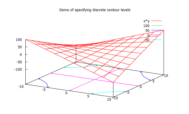
ChGnuPlot mplot("__tmp_gnuplot_1.gpl");
mplot << "set contour";
mplot << "set title 'Demo of specifying discrete contour levels'";
mplot << "splot x*y";

When the mplot object goes out of scope and is deleted at the end of this example, the script is saved on disk and GNUplot is launched.

You should see the following windows that opens:

Troubleshooting. If you do not see the window opening, check the following:
... if you open a shell (a DOS cmd window in Windows) and type gnuplot, does gnuplot start? If the program is not found, you should install gnuplot.
... make sure you can access it from the shell (add it to your PATH in windows)
... in case the .gpl command script contains errors, you can see which is the offending statement by opening a shell, go to the current working directory of the demo_POST_gnuplot executable using cd, and entering gnuplot __tmp_gnuplot_1.gpl where __tmp_gnuplot_1.gpl is the name of the gpl file, here is for this example. When executed it will prompt script errors, if any.

Example 2

Learn how to use the Open... functions to define the output terminal. The gnuplot utility can create plots in windows, or it can save them as EPS or JPG or PNG or other formats.

This is a demo that opens two plots in two windows and save the second to an EPS file too.

Note that we use SetGrid(), SetLabelX(), SetLabelY(). There are other functions like these. They are shortcuts to alleviate you from entering complex gnuplot commands. For instance mplot.SetLabelX("x"); is equivalent to mplot << "set xlabel \"x"";, etc.

ChGnuPlot mplot("__tmp_gnuplot_2.gpl");

mplot.SetGrid();

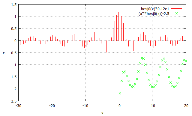
Then we redirect a first plot to a window n.0:

mplot.OutputWindow(0);
mplot.SetLabelX("x");
mplot.SetLabelY("y");
mplot << "plot [-30:20] besj0(x)*0.12e1 with impulses, (x**besj0(x))-2.5 with points";

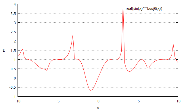
We redirect a following plot to a window n.1:

mplot.OutputWindow(1);
mplot.SetLabelX("v");
mplot.SetLabelY("w");
mplot << "plot [-10:10] real(sin(x)**besj0(x))";

Finally we redirect a plot to an .EPS Postscript file, that can be used, for example, in LaTeX documents. Note that here we do not issue another plot command, but we rather use Replot(), that repeats the last plot command (the one of the window n.1).

mplot.OutputEPS("test_eps.eps");

mplot.Replot(); // repeat last plot

You should see the following two plots in two separate windows:

Example 3

Learn how to use the Plot() shortcut functions, for easy plotting from a .dat file (an ascii file with column ordered data).

Of course you could do this by just adding gnuplot commands such as

mplot << "plot \"test_gnuplot_data.dat\" 1:2

etc., but the Plot() functions make this easier.

Step 1: create a .dat file with three columns of demo data:

std::ofstream mdatafile("test_gnuplot_data.dat");
for (double x = 0; x<10; x+=0.1)
   mdatafile << x << ", " << sin(x) << ", "  << cos(x) << std::endl;

Step 2: Create the plot.

Note the Plot() shortcut: In this case you pass the .dat filename, the columns IDs, title and custom settings that define the plotting line type, width, etc. (see the gnuplot documentation)

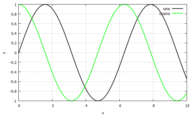
ChGnuPlot mplot("__tmp_gnuplot_3.gpl");
mplot.SetGrid();
mplot.SetLabelX("x");
mplot.SetLabelY("y");
mplot.Plot("test_gnuplot_data.dat", 1,2, "sine",   " with lines lt -1 lw 2");

Note that you can have multiple Plot() calls for a single Output, they will be overlapped as when you use commas in gnuplot: plot ... , ... , .... For instance, here overlap a 2nd plot to the previous one:

mplot.Plot("test_gnuplot_data.dat", 1,3, "cosine", " with lines lt 2 lw 2");

You should see the following plot:

Example 4

To make things even simpler, the Plot() shortcut function can be used directly on embedded data, without needing to save a .dat file.

One can use, for instance:

a pair of x,y vectors (use chrono::ChVectorDynamic column matrices),
chrono::ChFunction y(x) objects,
chrono::ChFunctionInterp
columns from a chrono::ChMatrixDynamic, etc.

The data values will be saved embedded in the .gpl file.

Note, the Replot() command does not work with embedded data.

Let's begin with creating some example data:

//create demo data in a pair of x,y vectors
ChVectorDynamic<> mx(100);
ChVectorDynamic<> my(100);
for (int i=0; i<100; ++i)
{
    double x = ((double)i/100.0)*12;
    double y = sin(x)*exp(-x*0.2);
    mx(i)=x;
    my(i)=y;
}
// ..or create demo data in a ChFunctionInterp
ChFunctionInterp mfun;
for (int i=0; i<100; ++i)
{
    double x = ((double)i/100.0)*12;
    double y = cos(x)*exp(-x*0.4);
    mfun.AddPoint(x,y);
}
// ..or create demo data in two columns of a ChMatrix
ChMatrixDynamic<> matr(100,10);
for (int i=0; i<100; ++i)
{
    double x = ((double)i/100.0)*12;
    double y = cos(x)*exp(-x*0.4);
    matr(i,2)=x;
    matr(i,6)=y*0.4;
}

Now create the plot. Note the Plot() shortcuts.

ChGnuPlot mplot("__tmp_gnuplot_4.gpl");
mplot.SetGrid();
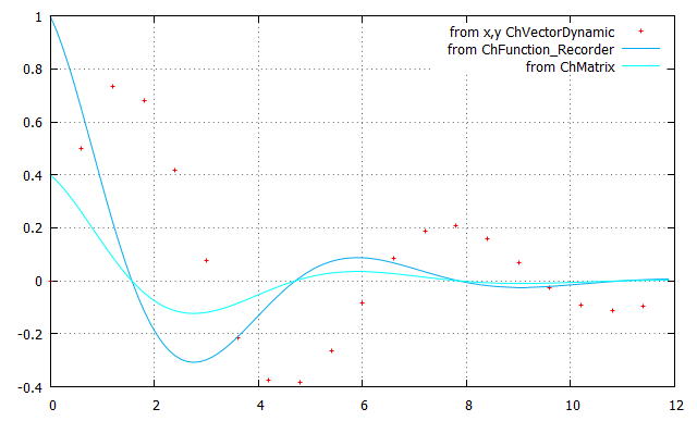
mplot.Plot(mx,my, "from x,y ChVectorDynamic",  " every 5 pt 1 ps 0.5");
mplot.Plot(mfun,  "from ChFunctionInterp",  " with lines lt -1 lc rgb'#00AAEE' ");
mplot.Plot(matr,   2,6, "from ChMatrix", " with lines lt 5");

You should see the following plot:

// =============================================================================
// PROJECT CHRONO - http://projectchrono.org
//
// Copyright (c) 2014 projectchrono.org
// All rights reserved.
//
// Use of this source code is governed by a BSD-style license that can be found
// in the LICENSE file at the top level of the distribution and at
// http://projectchrono.org/license-chrono.txt.
//
// =============================================================================
// Authors: Alessandro Tasora
// =============================================================================
//
// Demo on using GNUplot for plotting graphs
//
// =============================================================================
 
#include <cmath>
 
#include "chrono/core/ChGlobal.h"
#include "chrono/functions/ChFunctionInterp.h"
 
#include "chrono_postprocess/ChGnuPlot.h"
 
#include "chrono_thirdparty/filesystem/path.h"
 
using namespace chrono;
using namespace postprocess;
 
int main(int argc, char* argv[]) {
    std::cout << "Copyright (c) 2017 projectchrono.org\nChrono version: " << CHRONO_VERSION << std::endl;
 
    std::cout << "CHRONO demo that launches GNUplot for plotting graphs:\n" << std::endl;
 
    // Create (if needed) output directory
    const std::string out_dir = GetChronoOutputPath() + "DEMO_GNUPLOT";
    if (!filesystem::create_directory(filesystem::path(out_dir))) {
        std::cout << "Error creating directory " << out_dir << std::endl;
        return 1;
    }
 
    {
        //
        // EXAMPLE 1
        //
 
        // The most low-level way of using the ChGnuPlot class:
        // use the the SetCommand() or alternatively << , to build the script file.
 
        ChGnuPlot mplot(out_dir + "/tmp_gnuplot_1.gpl");
        mplot << "set contour";
        mplot << "set title 'Demo of specifying discrete contour levels'";
        mplot << "splot x*y";
 
        // When the mplot object goes out of scope and is deleted at the end of this example, the
        // script is saved on disk and GNUplot is launched.
    }
 
    {
        //
        // EXAMPLE 2
        //
 
        // Use the Open... functions to define the output terminal.
        // Open two plots in two windows and also save the second to EPS and PNG files.
        // Learn shortcut calls:
        //  SetGrid() to make a grid
        //  SetLabelX() SetLabelY() to setup labels
 
        ChGnuPlot mplot(out_dir + "/tmp_gnuplot_2.gpl");
        mplot.SetGrid();
 
        mplot.OutputWindow(0);
        mplot.SetLabelX("x");
        mplot.SetLabelY("y");
        mplot << "plot [-30:20] besj0(x)*0.12e1 with impulses, (x**besj0(x))-2.5 with points";
 
        mplot.OutputWindow(1);
        mplot.SetLabelX("v");
        mplot.SetLabelY("w");
        mplot << "plot [-10:10] real(sin(x)**besj0(x))";
 
        mplot.OutputEPS(out_dir + "/test_eps.eps");
        mplot.OutputPNG(out_dir + "/test_eps.png", 800, 600);
        mplot.Replot();  // repeat last plot
    }
 
    {
        //
        // EXAMPLE 3
        //
 
        // Learn the Plot() shortcut function, for easy plotting from a .dat file (ascii file
        // with column ordered data).
 
        // Step 1.
        // create a .dat file with three columns of demo data:
        std::string datafilename = out_dir + "/test_gnuplot_data.dat";
        std::ofstream datafile(datafilename);
        for (double x = 0; x < 10; x += 0.1)
            datafile << x << ", " << std::sin(x) << ", " << std::cos(x) << std::endl;
 
        // Step 2.
        // Create the plot.
        // NOTE. The plot shortcuts. In this case you pass the .dat filename, the columns IDs, title and custom settings
        // NOTE. You can have multiple Plot() calls for a single Output,
        // they will be overlapped as when you use commas in gnuplot:  "plot ... , ... , ..."
        ChGnuPlot mplot(out_dir + "/tmp_gnuplot_3.gpl");
        mplot.SetGrid();
        mplot.SetLabelX("x");
        mplot.SetLabelY("y");
        mplot.Plot(datafilename, 1, 2, "sine", " with lines lt -1 lw 2");
        mplot.Plot(datafilename, 1, 3, "cosine", " with lines lt 2 lw 2");
    }
 
    {
        //
        // EXAMPLE 4
        //
 
        // The Plot() shortcut function can be used directly on embedded data, without
        // needing to save a .dat file. One can use, for instance:
        //  - a pair of x,y vectors (use ChVectorDynamic column matrices)
        //  - ChFunction y(x) objects
        //  - columns from a ChMatrix
        // The values will be saved as embedded in the .gpl file.
        // Note, the Replot command does not work with embedded data.
 
        // create demo data in a pair of x,y vectors
        ChVectorDynamic<> mx(100);
        ChVectorDynamic<> my(100);
        for (int i = 0; i < 100; ++i) {
            double x = ((double)i / 100.0) * 12;
            double y = std::sin(x) * std::exp(-x * 0.2);
            mx(i) = x;
            my(i) = y;
        }
        // ..or create demo data in a ChFunctionInterp
        ChFunctionInterp mfun;
        for (int i = 0; i < 100; ++i) {
            double x = ((double)i / 100.0) * 12;
            double y = std::cos(x) * std::exp(-x * 0.4);
            mfun.AddPoint(x, y);
        }
        // ..or create demo data in two columns of a ChMatrix
        ChMatrixDynamic<> matr(100, 10);
        for (int i = 0; i < 100; ++i) {
            double x = ((double)i / 100.0) * 12;
            double y = std::cos(x) * std::exp(-x * 0.4);
            matr(i, 2) = x;
            matr(i, 6) = y * 0.4;
        }
 
        // Create the plot.
        // NOTE. The plot shortcuts.
        ChGnuPlot mplot(out_dir + "/tmp_gnuplot_4.gpl");
        mplot.SetGrid();
        mplot.Plot(mx, my, "from x,y ChVectorDynamic", " every 5 pt 1 ps 0.5");
        mplot.Plot(mfun, "from ChFunctionInterp", " with lines lt -1 lc rgb'#00AAEE' ");
        mplot.Plot(matr, 2, 6, "from ChMatrix", " with lines lt 5");
    }
 
    {
        //
        // EXAMPLE 5
        //
 
        // Example of subplot capability.
 
        // Step 1.
        // Create some data for plotting.
        ChVectorDynamic<> time = ChVectorDynamic<>::LinSpaced(20, 0, 6.28);
        ChVectorDynamic<> x = time.unaryExpr([](double ti) { return 3 * std::sin(2 * ti); });
        ChVectorDynamic<> xshift = time.unaryExpr([](double ti) { return 3 * std::sin(2 * ti + 1.2); });
        ChVectorDynamic<> x_t = time.unaryExpr([](double ti) { return 6 * std::cos(2 * ti); });
        ChVectorDynamic<> x_tt = time.unaryExpr([](double ti) { return -12 * std::sin(2 * ti); });
 
        // Step 2.
        // Create the plot.
        ChGnuPlot mplot(out_dir + "/tmp_gnuplot_5.gpl");
        mplot.OutputWindow(0);
        mplot.SetColorSequence(1); // change default color sequence
        //
        mplot.StartSubplot(3, 1, 0);
        mplot.SetGrid();
        mplot.SetLabelY("x");
        mplot.SetTitle("Position subplot");
        mplot.Plot(time, x, "x", "with lines lw 2");
        mplot.Plot(time, xshift, "xshift", "with lines lw 2");
        //
        mplot.StartSubplot(3, 1, 1);
        mplot.Plot(time, x_t, "", "with lines lw 2");
        mplot.SetGrid();
        mplot.SetLabelY("x_t");
        mplot.SetTitle("Velocity subplot");
        //
        mplot.StartSubplot(3, 1, 2);
        mplot.Plot(time, x_tt, "", "with lines lw 2");
        mplot.SetLabelX("Time");
        mplot.SetLabelY("x_{tt}");
        mplot.SetTitle("Acceleration subplot");
        //
        mplot.EndSubplot();
    }
 
    std::cout << "\nCHRONO execution terminated.";
 
    return 0;
}