Introduction
Deep Reinforcement Learning (DRL) consits in using Reinforcement Learning to train Deep Neural Network. In the last few years it has been applied with success to various robotic control tasks. The main advantage of this approach is its ability to deal with unstructured and mutable environments, while classical robotic control often fails when facing these challenges. To train a NN with DRL several interactions with the environment are needed. For this reason physical engines offer a valuable help, allowing to train the agent in a virtual environment instead of training it directly in the real world, reducing time and risks of the operation. With PyChrono you can easily build physical models and exchange data between the simulation and you favorite ML framework. We suggest two ways to get started using PyChrono for DRL:
1- gym-chrono
If you are looking for more complex and realistic environments and you want to leverage OpenAI Gym capabilities (i.e. using OpenAI Baselines) we recommend to use gym-chrono, a set of PyChrono-based OpenAI Gym environments. These environments provide an open-source alternative to MuJoCo environments.
2- Tensorflow Demos
We also provide 2 simple plug-and-play examples to kickstart you into DRL for robotic control. These demos only require Tensorflow and PyChrono to run; and are provided together with a standalon Proximal Policy optimization algorithm.
Requirements:
In order to run these demos, you will need:
- Numpy
- Scikit-Learn
- Tensorflow 1
We recommend to use Anaconda. To prepare your environment do the following:
- Download and install Anaconda. We suggest user-only installation and to set Anaconda as your default Python.
- Create a new Python environment. If you've built PyChrono from sources, set the Python version of your environment as the version of the Python executable you pointed to in CMake. You could also use the executable, headers and libraries of the virtual environment to build PyChrono.
- Activate the new environment
- If you have not built from sources, install pychrono using Anaconda conda install -c projectchrono pychrono
- Install Numpy conda install numpy
- Install Scikit-Learn conda install scikit-learn
- Install Tensorflow conda install tensorflow-gpu=1.14
Goal:
We will train a Neural Network to solve robotic tasks using virtual training environment created with PyChrono. The demo contains virtual environments and a learning model created with Tensorflow.
Environments
We provide two sample environments for robotic control.
ChronoPendulum
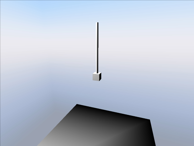
Inverted pendulum, the goal is to balance a pole on a cart. 1 action (force along the z axis) and 4 observations (position and speed of cart and pole).
ChronoAnt
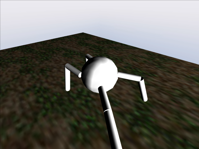
A 4-legged walker, the goal is learning to walk straight as fast as possible. 8 actions (motor torques) and 30 observations.
DL algorithm
To train the Neural Networks to solve the tasks we used a reinforcement learning algorithm known as Proximal Policy Optimization (PPO). PPO is an on-policy actor-critic algorithm, thus you will find 2 NNs: the first one given the state prescribes an action (Policy), the second given the state evaluates the value function (VF).
The policy and value function codes are in the Policy.py and VF.py respectively.
How to run examples
Make sure that you are using the right Python interpreter (the one with Pychrono an Tensorflow installed). Then simply run the script with the needed keyboard arguments
Serial and Parallel Training
You can choose between "train_serial.py" and "train_parallel.py". The parallel version collects data over multiple simulations using the Python multiprocessing module. In the advanced stages of training, when episodes last longer, this feature greatly speeds up the learning process.
EXAMPLES:
Train the inverted pendulum over 1000 episodes:
Train the 4-legged ant to walk over 20000 episodes:
Alternatively, launch the demo from your favorite IDE, but remember to add the required arguments.
List of command line arguments
Besides the environment name and the number of episodes, there are some other arguments, mainly to hand-tune learning parameters. ** –renderON/–renderOFF ** toggles on and off the simulation render. Consider that visualizing the render will slow down the simulation and consequentially the learning process.
- Environment name :
env_name - Number of episodes:
-n,--num_episodes, default=1000 - Run-time visualization:
--renderON/--renderOFF - Discount factor:
-g,--gamma, default=0.995 - Lambda for GAE:
-l,--lam, default=0.98 - Kullback Leibler divergence target value:
-k,--kl_targ, default=0.003 - Batch size:
-b,--batch_size, default=20
Saving and restoring
NN parameters and the other TF variables are stored inside the Policy and VF directories, while the scaler means and variances are stored in the scaler.dat saved numpy array. These files and folders are stored and used to restore a previous checkpoint.
Since they use the same NN architecture using parallel or serial version does not matter when restoring checkpoints.
Tester
To test the Policy without further improving it, execute tester.py. Set --VideoSave to save screenshots from the render.