Table of Contents
A terrain object in Chrono::Vehicle must provide methods to:
- return the terrain height at a specified \((x,y)\) location
- return the terrain normal at a specified \((x,y)\) location
- return the terrain coefficient of friction at at a specified \((x,y)\) location
See the definition of the base class ChTerrain.
Note however that these quantities are relevant only for the interaction with the so-called semi-empirical tire models. As such, they are not used for the case of deformable terrain (SCM, granular, or FEA-based) which can only work in conjunction with rigid or FEA tire models and with tracked vehicles (as they rely on the underlying Chrono collision and contact system).
Furthermore, the coefficient of friction value may be used by certain tire models to modify the tire characteristics, but it will have no effect on the interaction of the terrain with other objects (including tire models that do not explicitly use it).
The ChTerrain base class also defines a functor object ChTerrain::FrictionFunctor which provides an interface for specification of a position-dependent coefficient of friction. The user must implement a custom class derived from this base class and implement the virtual method operator() to return the coefficient of friction at the given \((x,y)\) location.
Flat terrain
FlatTerrain is a model of a horizontal plane, with infinite \(x\) and \(y\) extent, located at a user-specified \(z\) height. The method FlatTerrain::GetCoefficientFriction returns the constant coefficient of friction specified at construction or, if a FrictionFunctor object was registered, its return value.
Since the flat terrain model does not carry any collision and contact information, it can only be used with the semi-empirical tire models.
Rigid terrain
RigidTerrain is a model of a rigid terrain with arbitrary geometry. A rigid terrain is spcified as a collection of patches, each of which can be one of the following:
- a rectangular box, possibly rotated; the "driving" surface is the \(+z\) face of the box
- a triangular mesh read from a user-specified Wavefront OBJ file
- a triangular mesh generated programatically from a user-specified gray-scale BMP image
The rigid terrain model can be used with any of the Chrono::Vehicle tire models, as well as with tracked vehicles.
A box patch is specified by its 3 dimensions (a 3D vector which encodes the length, width, and height, respectively) and the box orientation (a coordinate system which defines the box center and its orientation). Optionally, the box patch can be created from multiple adjacent tiles, each of which being a Chrono box contact shape; this is recommended for a box patch with large \((x,y)\) extent as a single collision shape of that dimension may lead to errors in the collision detection algorithm.
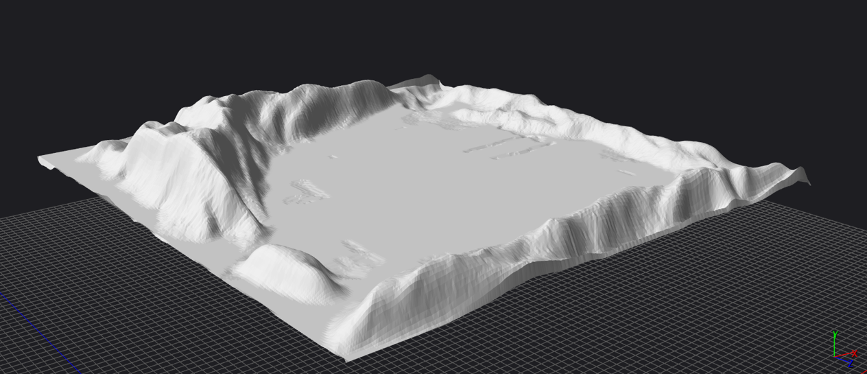
An example of a mesh rigid terrain patch is shown in the image below. It is assumed that the mesh is provided with respect to an ISO reference frame and that it has no "overhangs" (in other words, a vertical ray intersects the mesh in at most one point). Optionally, the user can specify a "thickness" for the terrain mesh as the radius of a sweeping sphere. Specifying a small positive value for this radius can significantly iprove the robustness of the collision detection algorithm.
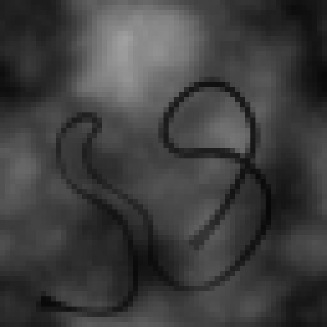
A height-map patch is specified through a gray-scale BMP image (like the one shown below), a horizontal extent of the patch (the \(x\) and \(y\) dimensions), and a height range (minimum and maximum heights). A triangular mesh is programatically generated, by creating a mesh vertex for each pixel in the input BMP image, stretching the mesh in the \((x,y)\) plane to match the given horizontal extent and in the \(z\) direction such that the minimum height corresponds to a perfectly black pixel color and the maximum height corresponds to a perfectly white pixel.
Height and normal calculation. The implementation of RigidTerrain::GetHeight and RigidTerrain::GetNormal rely on a relatively expensive ray-casting operation: a vertical ray is cast from above in all constituent patches with the height and normal at the intersection point reported back. For a box patch, the ray-casting uses a custom analytical implementation which finds intersections of the ray with the \(+z\) face of the box domain; for mesh-based patches, the ray-casting is deferred to the underlying collision system. If no patch is intersected, these functions return \(0\) and \([0,0,1]\), respectively.
Location-dependent coefficient of friction. The rigid terrain model supports the definition of a FrictionFunctor object. If no such functor is provided, RigidTerrain::GetCoefficientFriction uses the ray-casting approach to identify the correct patch and the (constant) coefficient of friction for that patch is returned. If a functor is provided, RigidTerrain::GetCoefficientFriction simply returns its value. However, processing of contacts with the terrain (e.g., when using rigid tires or a tracked vehicle) is relatively expensive: at each invocation of the collision detection algorithm (i.e., once per simulation step) the list of all contacts in the Chrono system is traversed to intercept all contacts that involve a rigid terrain patch collision model; for these contacts, the composite material properties are modified to account for the terrain coefficient of friction at the point of contact.
A rigid terrain can be constructed programatically, defining one patch at a time, or else specified in a JSON file like the following one:
CRG terrain
CRGTerrain is a procedural terrain model constructed from an OpenCRG road specification. To use this terrain model, the user must install the OpenCRG SDK and enable its use during CMake configuration (see the Chrono::Vehicle installation instruction).
The CRG terrain creates a road profile (a 3D path with an associated width) from a specification file such as the one listed below and implements the functions CRGTerrain::GetHeight and CRGTerrain::GetNormal to use this specification. Note that a crg specification file can be either ASCII or binary.
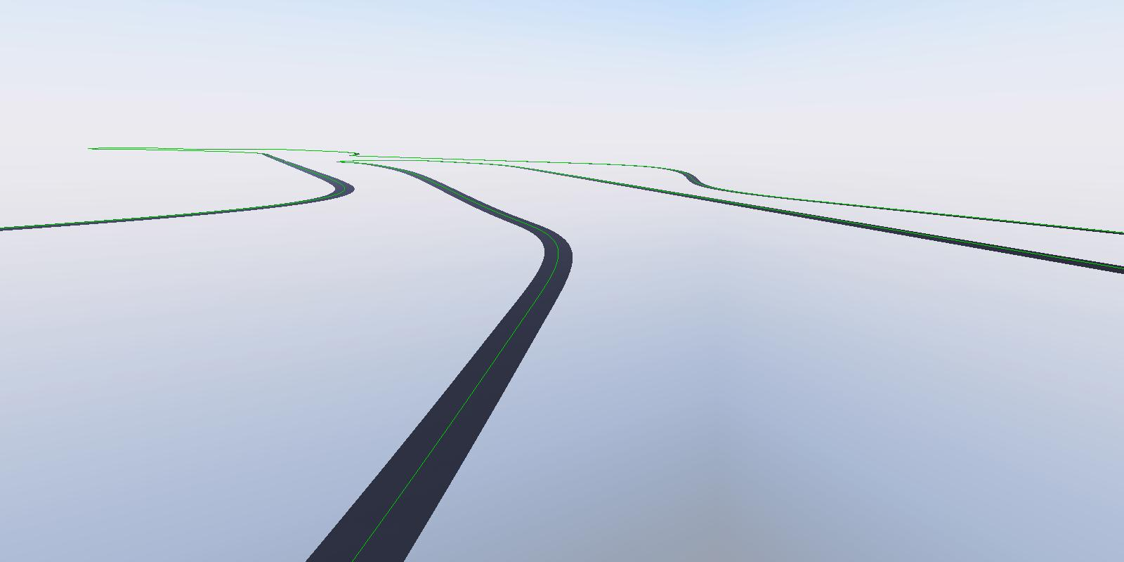
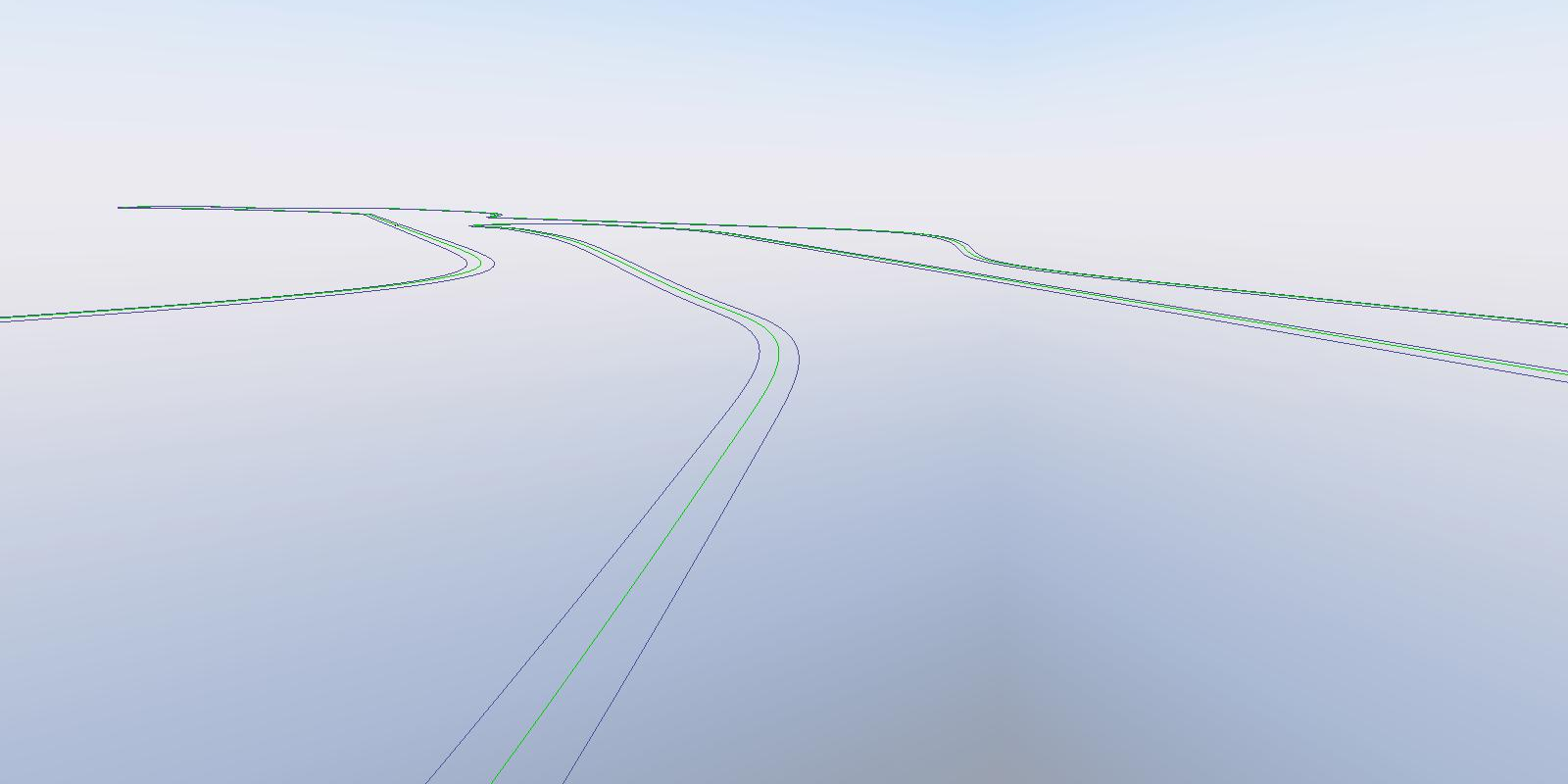
The CRG terrain can be visualized as a triangular mesh (representing the road "ribbon") or else as a set of 3D Bezier curves (representing the center line and the road sides). Other features of CRGTerrain include:
- ability to export the road mesh (as a triangle mesh)
- ability to export the center line (as a Bezier curve)
- methods for reporting the road length and width
The images below illustrate the run-time visualization of a CRG road using a triangular mesh or the road boundary curves.
Since the CRG terrain model currently does not carry any collision and contact information, it can only be used with the semi-empirical tire models.
Deformable SCM (Soil Contact Model)
In SCM, the terain is represented by a mesh whose deformation is achieved via vertical deflection of its nodes. Differently from the original SCM model, which uses regular grids, Chrono's SCMDeformableTerrain extends this model to the case of non-structured triangular meshes. Moreover, to address memory and computational efficiency concerns, the Chrono implementation uses an automatic refinement of the mesh in order to create additional fine details where vehicle tires and track shoes interact with the soil. This soil model draws on the general-purpose collision engine in Chrono and its lightweight formulation allows computing vehicle-terrain contact forces in close to real-time.
An illustration of the adaptive mesh refinement implemented in the Chrono version of the SCM is shown below:

SCM is based on a semi-empirical model with few parameters, which makes it easy to calibrate based on experimental results. It can be considered a generalization of the Bekker-Wong model to the case of wheels (or track shoes) with arbitrary three-dimensional shapes. The Bekker formula for a wheel that moves on a deformable soil provides a relationship between pressure and vertical deformation of the soil as:
\[ \sigma = \left( \frac{k_c}{b} + k_{\phi} \right) y^n \]
where \(\sigma\) is the contact patch pressure, \(y\) is wheel sinkage, \(k_c\) is an empirical coefficient representing the cohesive effect of the soil, \(k_{\phi}\) is an empirical coefficient representing the stiffness of the soil, and \(n\) is an exponent expressing the hardening effect, which increases with the compaction of the soil in a non-linear fashion. Finally, \(b\) is the length of the shorter side of the rectangular contact footprint (since the original Bekker theory assumes a cylindrical tire rolling over flat terrain).
For a generic contact footprint, the length \(b\) cannot be interpreted as in the original Bekker model; instead, we estimate this length by first obtaining all connected contact patches (using a flooding algorithm) and the using the approximation
\[ b \approx \frac{2 A}{L} \]
where \(A\) is the area of such a contact patch and \(L\) its perimeter.
Some other features of the Chrono SCM implementation are:
- the initial undeformed mesh can be created as
- a regular tiled mesh (filling a flat rectangle)
- an arbitrary triangular mesh (provided as a Wavefront OBJ file)
- from a hight-map (provided as a gray-scale BMP image)
- programatically
- support for arbitrary orientation of the terrain reference plane; by default, the terrain is defined as the \((x,y)\) plane of a \(z\)-up ISO frame
- support for a moving-patch approach wherein the adaptive mesh refinement is confined to a rectangular domain around a given point on a moving vehicle
- support for specifying location-dependent soil parameters; this can be achieved by providing a custom callback class which implements a method that returns all soil parameters at a given \((x,y)\) point specified in the terrain's reference plane. See SCMDeformableTerrain::SoilParametersCallback
Since the interaction with this terrain type is done through the underlying Chrono contact system, it can be used in conjunction with rigid or FEA tire models and with tracked vehicles.
Granular terrain
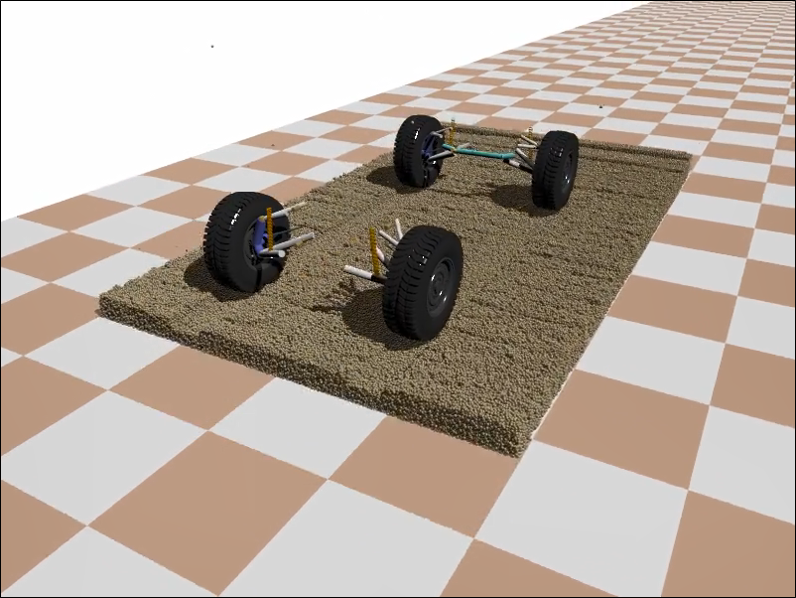
GranularTerrain implements a rectangular patch of granular material and leverages Chrono's extensive support for so-called Discrete Element Method (DEM) simulations. Currently, this terrain model is limited to monodisperse spherical granular material.
Because simulation of large-scale granular dynamics can be computationally very intensive, the GranularTerrain object in Chrono::Vehicle provides support for a "moving patch" approach, wherein the simulation can be confined to a bin of granular material that is continuously relocated based on the position of a specified body (typically the vehicle's chassis). Curently, the moving patch can only be relocated in the \(x\) (forward) direction.
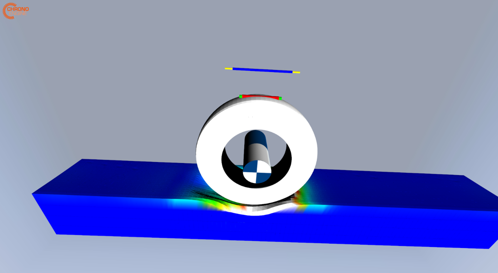
An illustration of a vehicle acceleration test on GranularTerrain using the moving patch feature is shown below. This simulation uses more than 700,000 particles and the Chrono::Parallel module for multi-core parallel simulation.
Other features of GranularTerrain include:
- generation of initial particle locations in layers, with particle positions in the horizontal plane uniformly distributed and guaranteed to be no closer than twice the particle radius
- inclusion of particles fixed to the bounding bin (to inhibit sliding of the granular material bed as a whole); due to current limitations, this feature should not be used in conjunction with the moving patch option
- analytical definition of the bin boundaries and a custom collision detection mechanism
- reporting of the terrain height (defined as the largest \(z\) value over all particle locations)
Since the interaction with this terrain type is done through the underlying Chrono contact system, it can be used in conjunction with rigid or FEA tire models and with tracked vehicles.
Deformable FEA (ANCF solid elements)
FEADeformableTerrain provides a deformable terrain model based on specialized FEA brick elements of type ChElementBrick_9.
This terrain model permits:
- discretization of a box domain into a user-prescribed number of elements
- assignment of material properties (density, modulus of elasticity, Poisson ratio, yield stress, hardening slope, dilatancy angle, and friction angle)
- addition of Chrono FEA mesh visualization assets
Since the interaction with this terrain type is done through the underlying Chrono contact system, it can be used in conjunction with rigid or FEA tire models and with tracked vehicles.